Donnerstag, 7. Juli 2016

Python: Concate code to a single string

Using the code below, the code from a source file can be concatenated to a single string. This string however can still be printed and formates nicely on a JavaScript console. It returns a string variable `s' and requires two command line arguments.
# Usage:
# > python ~/path/to/script/multiline.py <name_of_ouput_variable>  
    filename = sys.argv[1]
    
    f = open(filename, "r")
    d = f.readlines()
    f.close()
    
    s = "var %s = " % sys.argv[2]
    s = s.strip()
    
    # s += '"' + "".join(d).replace("\n", "") + '";'

    cnt = 0
    n = len(d)

    # '\\n' is explicitly written to the 'source'-file such that
    # the JavaScript console can print the source code including line
    # breaks.
    for line in d:
        # First line.
        if cnt == 0:
            s += "\n" + '  "' + d[cnt].replace("\n", "") + '\\n"\n'
            cnt += 1
        # Inbetween lines.
        elif cnt > 0 and cnt < (n-1):
            s += '+ "' + d[cnt].replace("\n", "") + '\\n"\n'
            cnt += 1
        # Last line.
        else:
            s += '+ "' + d[cnt].replace("\n", "") + '"'

Sonntag, 1. Mai 2016

R: Replacement functions

If you use R, you've been using so called replacement functions such as '<-' to assign a value to a variable or 'colnames' to define names of columns in a data frame.
Remember, in R everything operation is a function call (therefore also the assignment operations).
In the following, the behaviour of the replacement functions are illustrated (and compared to a -failing- ordinary approach) and code is shown to list all replacement functions in the base R package.

Replacement functions act as if they modify their arguments in place such as in

colnames(d) <- c("Input", "Output")

They have the identifier '<-' at the end of their name and return a modified copy of the argument object (non-primitive replacement functions) or the same object (primitive replacement functions).

At the R prompt, the following will not work:

> `second` <- function(x, value) {
+   x[2] <- value
+   x
+ }
> x <- 1:10
> x
 [1]  1  2  3  4  5  6  7  8  9 10
> second(x) <- 9
Fehler in second(x) <- 9 : konnte Funktion "second<-" nicht finden


As one can see, behind the scenes, R is looking for a function called 'second<-'. So lets do the same thing but using this name:

> `second<-` <- function(x, value) {
+   x[2] <- value
+   x
+ }


Now, the assignment at the second position of the vector works:

> second(x) <- 9
> x
 [1]  1  9  3  4  5  6  7  8  9 10


The following code allows to list all replacement functions in are and check if they are primitive:


# Get all objects from the base package, then
# functions from among those objects.
objs <- mget(ls("package:base"), inherits=TRUE)
funs <- Filter(is.function, objs)
 
# Replacement functions have '<-' at the end of their name.
get_rep_fun <- function(fun_i) {
  if(substr(fun_i, nchar(fun_i) - 1, nchar(fun_i)) == "<-") {
    fun_i
  }
}
 
# The list returned by 'lapply' contains many 'NULL'
# entries. Only non-'NULL' function name strings remain
# after 'unlist'.
rep_funs <- lapply(names(funs), get_rep_fun)
rep_funs <- unlist(rep_funs)
 
# Identify primitive replacement functions.
get_prim_rep_fun <- function(rep_fun) {
  if(is.primitive(rep_fun)) {
    rep_fun
  }
}
 
# Get the actual function object by 'sapply'-ing 'get' to
# each string identifier from the 'rep_funs' vector.
prim_rep_funs <- lapply(sapply(rep_funs, get), is.primitive)
 
# Prepare data frame for convenience.
k <- data.frame(fun_name = rep_funs, prim=unlist(prim_rep_funs))
 
# Rows are named after functions -> reduce redundancy.
rownames(k) <- NULL


Sonntag, 3. April 2016

Clustering data with k-means and plotting for exploratory analysis

I clustered data from my paper A computational method for the systematic screening of reaction barriers in enzymes: searching for Bacillus circulans xylanase mutants with greater activity towards a synthetic substrate using k-means clustering and plotted the results using the `Lattice` library in R.
This analysis could be used to further automate selection of reaction barriers for including or excluding from analysis if the barrier profile is not physically meaningfull.

Raw data:
http://pastebin.com/41TrNNvH

A detailed report on the analyis is available here:
http://rpubs.com/mzh/167769

Github repository:
https://github.com/mzhKU/Enzyme-Barrier-Clustering

The critical part of the code is where the two plots (the k-means clusters, red lines, and the raw data of each cluster, blue lines) are overlayed using the lattice panel plot construct (in 003_execute.r):

# 'group' required to prevent drawing of a continuous line connecting the last
# data point of a mutant with the first data point of the next mutant barrier.
xyplot(Barrier_Cl ~ x|Cluster_fac, data=kmdf, iedf_i=iedf,
       ylim=c(-20, 50), ylab="Reaction Energy [kcal/mol]",
       xlab="Reaction Coordinate", xlim=c(1, 12), strip=T,
       # Note:
       # 'x' and 'y' are the data from the cluster data frame 'kmdf'.
       # 'iedf_i' is the 'iedf'-data frame provided to the 'i'-nner panel function.
       panel = function(x, y, iedf_i)
       {
            panel.xyplot(x=iedf_i[iedf_i$Cluster==panel.number(), ]$x_axis,
                         y=iedf_i[iedf_i$Cluster==panel.number(), ]$Barrier_i,
                         group=iedf_i$id, subscripts=TRUE, type="o", col="blue")
            panel.xyplot(x, y, type="l", col="red", lwd=2)
       }
)

Sonntag, 20. September 2015

Literature 004: Jinek et al., eLife 2013; 2:e00417


Introduction

CRISPRs have attracted enormous attention since the recent publication by Jinek et al. The discovery has been subject to numerous reviews in both the scientific literature as well as popular and mass media publications:
  • The Economist ("[...]where doctors put normal genes into the cells of people who suffer from genetic diseases such as Tay Sachs or cystic fibrosis."- note how simply doctors these days just "put" normal genes into the cells of people, of course only the right cells... you've had yours today already, haven't you?)
While providing information to the public about this discovery is of tremendous importance, many reports however seem to emphasize promising future applications without giving any understanding of how this development actually looked like when it was made in the laboratory. I.e. the real data obtained by the scientists in those breakthrough moments is rarely if ever shown.
The eLife publication is open access so it can't be a mather of accessibility. Much rather I believe journalists prefer to present fancy 3d-renderings of DNA and proteins with fluorescent numbers and pseudo-code on a black background, like everything was in Matrix or so - for whatever reason. But, the real science is actually just as appealing and therefore in this post, the real data is shown and explained.


Background

Subject of interest is a protein-RNA complex which can cut dsDNA at virtually any position and which is much cheaper and easier to use than any of the sofar existing methods. This complex is called the CRISPR/Cas-9 system and it was discovered 1987[Ishino et al.] when its involvement in cutting dsDNA was yet completely unclear.
The discovery back then looked like this:
A pattern is immediatly visible (the point being science is not always that difficult).
The underlined repeats are of dyadic symmetry and regularly separated by (non-uniform) short spacer sequences. The authors wrote:
This structure was "unusual" to them. I can only imagine how much time they spent wondering what this was about before they wrote this paragraph.

Only 2004/2005 was it recognized that the non-uniform sequences were from foreign DNA.[Pourcel el al., Mojica et al., Bolotin et al.] The random looking sequences to the right of the dyadic elements in the above figure are the foreign DNA fragments of previous viral attacks on the cell. The dyadic elements are also referred to as palindromic because they can be folded and basepaired onto themselves.
Gradually, attention was rising and in 2010 the first Science and Nature reviews on the topic appeared.[Horvath et al., Marraffini et al.] Application to dsDNA was alluded to at that point, but nothing was certain.
"[...]Other potential applications of CRISPRs await fur­ ther development to determine their plausibility. For example, a crRNP complex in P. furiosus50 can cleave a target RNA at a specific site dictated by the sequence of the crRNA guide. This activity could in principle have applications in molecular biology to specifically cleave RNA molecules in vitro, and could be extended to DNA molecules if other crRNP complexes are proven to have DNA endonuclease activity.[...]"
Remarkably, neither of these reviews cites any work by either Jinek, Doudna or Charpentier.
Then the two breakthrough papers were published.[Jinek et al. 2012, Jinek et al. 2013] In the following, the results of the 2013 paper are summarized.

The Jinek Publication

In the following, all images are taken from the eLife publication to show how the results lead to conclusions. Assume as a scientist, you don’t know in detail how the CRISPR/Cas9 system works and what you can use it for. All you know is it has to be transfered to the nucleus and is programmed by RNA. How can you prove your claim?
In the publication, the target gene is a clathrin gene, a protein participating in vesicle formation at the cell surface. Clathrin was subject to an earlier post on this blog.

First, its good to show that the protein of interest can indeed be expressed by the target (human) cells.
http://elifesciences.org/content/2/e00471
The black line at 170 kDa indicates a protein of roughly the weight one would expect for Cas9 being modified by a CMV promoter, an HA epitope (facilitating detection/purification), a nuclear localization signal (NLS) and a fluorescent signal (GFP).  This experiment proves that transfection of human embryonic kidney cells with the Cas9 construct works and that cells express the desired protein. Of course, the cell could be expressing other proteins with similar weight, but this experiment makes it highly plausible that the results of the subsequent experiments are indeed due to the Cas9 activity.


Then, since the protein is believed to be active in the nucleus where the DNA is, can it be shown that the protein gets to the nucleus after human embryonic kidney cells ("HEK293T cells") have been transfected with a DNA-fragment („vector“) encoding the above construct?
The below images show separately the GFPs, the cells and an overlay. It is not easy to see but it appears as if the GFPs shine from within the cell nucleus, and therefore most likely the Cas9 is also in the nucleus.

http://elifesciences.org/content/2/e00471

Especially the GFP image of four cells in the left bottom corner nicely overlaps with their nucleus position.

Now, since RNA is required to program the nuclease, can the target HEK cell express the guiding RNA while at the same time be transfected with engineered Cas9?

A Northern blot shows that indeed, third column from the left, guiding RNA („CLTA1 sgRNA“) of 62 nucleotide length (= 20 nt of guiding RNA + 42 nt of RNA required to bind the Cas9) is expressed by the cells.
http://elifesciences.org/content/2/e00471
In the fourth column from the left ("CLTA1 sgRNA + Cas9"), the signal is even a bit stronger, suggesting the stabilization of the sgRNA by Cas9. Possibly binding of the sgRNA by Cas9 protects it from degradation.

So, the pieces are in place. The cells can be transfected and they're shown to transcribe sgRNA and translate foreign Cas9 simultaneously. It remains to show that Cas9 is operative.


What happens to the DNA if the sgRNA and Cas9 together are expressed in a cell?
Transfecting HEK293T cells with a Cas9 vector and a vector for Clathrin directing sgRNA followed by isolation of cell products resulted in the following cell-lysate image.
http://elifesciences.org/content/2/e00471
For the moment, only consider columns under the "Cas9-mCherry" label. In all of these columns Cas9 is present (mCherry is another fluorescent labeling function).
To demonstrate the workings of Cas9, the authors use the so called Surveyor Assay method. This method allows to identify breaks in double stranded DNA, albeit only indirectly. When an agent like Cas9 breaks dsDNA the cell immediately fixes the DNA using its own fixing mechanisms (like non-homolguous end joining, NHEJ). These mechanisms are however error prone and can introduce mismatches, just like a genomic scar.
In the Surveyor assay then, the transfected cells are lysated and the DNA is extracted, amplified with PCR and then incubated in vitro with the nuclease Cel-1. This protein identifies mismatches resulting from NHEJ and again breaks the dsDNA at these positions. The products of this subsequent nuclease activity are what is analysed finally and shown in the above figure.
In the figure above then, the authors show step-by-step what effect only Cas9, sgRNA + Cas9, sgRNA + Cas9 + Cel-1 have, respectively.
If there is only Cas9 present (column 2, -/-), DNA of roughly 400 bp is found. Only Cas9 + Cel-1 again yields DNA of 400 bp. sgRNA + Cas9 also 400 bp (important: Cas9 was active here but in the absence of Cel-1 mismatches are not recognized). But then, in column 5 (+/+), a dim line at little less than 200 bp is visible. This dim line is what the whole excitement is about. The column with only sgRNA and Cas9 can be viewed as the control for the column with sgRNA, Cas9 and Cel-1 since it could be that Cel-1 itself has some sort of nuclease activity and cleaves DNA. But no, the third column (-/+) is negative.
A positive confirmation is provided by comparison to the ZFN results. ZFN is a highly engineered, very expensive system that cuts at almost the same position in the DNA.

From the image, the next question immediately arises: How can the dim line be made stronger?

Is there enough Cas9? Is there enough sgRNA? Does the sgRNA bind sufficiently strongly to Cas9? Should the guiding sequence be longer?
Checking for sgRNA availability, the authors found this:
http://elifesciences.org/content/2/e00471
When adding additional sgRNA, in column 5 (Cas9-HA-NLS-GFP plasmid + in vitro transcribed CLTA1 sgRNA added to lysate), the lines are indeed stronger. Even stronger than the ZFN signal. Here, the authors first transfected cells with Cas9 and sgRNA plasmids (just like before). The cells were then lysated (so the Cas9 protein was available in vitro) and then mixed with additional sgRNA. The signal gets stronger. So more sgRNA is better, however this doesn't explain why, is it because then overall there is more active Cas9? Or is it just because expression of plasmid sgRNA is not efficient enough?
The authors just added even more sgRNA:
http://elifesciences.org/content/2/e00471
The signal is strongest when both the sgRNA transcribed from plasmids as well as in vitro transcribed sgRNA are added to the system (right-most column).
It is concluded that either sgRNA expression or its loading into Cas9 is the limiting factor of Cas9 nuclease performance.

At the time of doing these experiments, probably the simplest second thing to do was to extend the region of sgRNA which is involved in binding to Cas9. So they did.
http://elifesciences.org/content/2/e00471
V1.0 represents the originally used system. In v2.1, the presumed Cas9 binding region is extended by 4 basepairs (red basepairs to the right of GAA) and the 3'-end was extended by 5 nucleotides. In v2.2, the Cas9 binding region was extended by 10 basepairs and the 3'-region by 5 nucleotides (compared to v1.0).
Again, a Surveyor Assay was carried out.
http://elifesciences.org/content/2/e00471
The results are not as clear as in the above case. Overall, v2.1 and v2.2 appear to have similar performance over v1.1 (7 - 8 % cleavage to 4 % cleavage in v1.1). This means that increasing the Cas9 binding region is more important than increasing the 3'-region of the sgRNA. Extension of the guiding sequence length was not examined. Furthermore, RNA can be stabilized in vivo by modifications at the 5'- or 3'-ends, both of which have not been further examined in these experiments.
The authors suggest more research in this direction to be necessary.

Finally, the above results are all in agreement with a visual model like this:
http://elifesciences.org/content/2/e00471

Discussion
Hopefully, the above could provide some understanding of the research and make the paper more accessible. In any case it will be interesting to see where this leads.
However, and this is very important to consider: what are the ethical implications of this technology. Given superb selectivity and sensitivity, the system could hypothetically be used to engineer the genome of living humans at will (and these changes could be inherited by later generations).
It is not yet conceivable, when the first genome engineering applications will be studied in clinical trials. To put it differently, who would want something injected that has the sole purpose of cutting the host DNA? Let it be clear that to date the only „test“ in a (disfunctional) single-cell human embryo was not perfectly successful[Liang et al.]:
"[...]Off-target cleavage was also apparent in these 3PN zygotes as revealed by the T7E1 assay and whole-exome sequencing.[...]".
Most recently, in April 2015, at a conference in California a number of leading geneticists met to discuss the implications of Cas9-based technology. In a perspectives publication, the authors end by strongly recommending against "...germline genome modifications for clinical applications  in humans as long as societal, environmental and ethical implications of such activity..." are not conclusively discussed.

It is left to hope that these recommendations are being taken into account by researchers when starting new Cas9 based research.


Edit (01. May, 2016):
A version of this post has been published on the blog of the Swiss based Think-Tank REATCH (Research and Technology in Switzerland).


Samstag, 3. Januar 2015

Excel like PivotTable and more with R


A table contains values as below (download from link under figure):


Item Category Price Profit Actual Profit Calories
Beer Beverages  $4.00 50%  $2.00 200
Soda Beverages  $2.50 80%  $2.00 120
Chocolate Bar Candy  $2.00 75%  $1.50 255
Ice Cream Sandwich Frozen Treats  $3.00 67%  $2.00 240
Bottled Water Beverages  $3.00 83%  $2.50 0
Gummy Bears Candy  $2.00 50%  $1.00 300
Soda Beverages  $2.50 80%  $2.00 120
Hamburger Hot Food  $3.00 67%  $2.00 320
Popcorn Hot Food  $5.00 80%  $4.00 500
Licorice Rope Candy  $2.00 50%  $1.00 280
Hot Dog Hot Food  $1.50 67%  $1.00 265
Licorice Rope Candy  $2.00 50%  $1.00 280
Popcorn Hot Food  $5.00 80%  $4.00 500

It is very easy to summarize the data using the Excel PivotTable generator (even for multiple variables like "Profit" and "Actual Profit" simultaneously):
Example taken from the Data Smart book.


It probably doesn't make a lot of sense to summarize the data by percentage, but this is just for illustration purposes.


A similar operation is the aggregate function in R (the Concessions.xlsx data frame is loaded as con):
> aggregate(cbind(Profit, Actual.Profit) ~ Category, data=con, FUN=sum)
       Category   Profit Actual.Profit
1     Beverages 31.23333          98.5
2         Candy 23.25000          46.5
3 Frozen Treats 23.00000          69.0
4      Hot Food 45.21667         142.0


The same is possible using the xtabs function:
> xtabs(cbind(Profit, Actual.Profit) ~ Category, data=con)
              
Category           Profit Actual.Profit
  Beverages      31.23333      98.50000
  Candy          23.25000      46.50000
  Frozen Treats  23.00000      69.00000
  Hot Food       45.21667     142.00000


Note, no special operation FUN is specified in xtabs.

Occurence of items can be done when specifing "Count" in the PivotTable builder:

R can do this with the plyr package and its count function.

> count(con$Item)
                       x freq
1                   Beer   20
2          Bottled Water   13
3          Chocolate Bar   13
4  Chocolate Dipped Cone   11
5            Gummy Bears   14
6              Hamburger   16
7                Hot Dog   15
8     Ice Cream Sandwich   10
9          Licorice Rope   13
10                Nachos   15
11                 Pizza   17
12               Popcorn   16
13              Popsicle   13
14                  Soda   13


This can also be done using the extremely powerful built-in functions of the data.table type:

> con[, .N, by=Item]
                     Item  N
 1:                  Beer 20
 2:         Bottled Water 13
 3:                  Soda 13
 4:         Chocolate Bar 13
 5:           Gummy Bears 14
 6:         Licorice Rope 13
 7:              Popsicle 13
 8:    Ice Cream Sandwich 10
 9: Chocolate Dipped Cone 11
10:               Popcorn 16
11:             Hamburger 16
12:                Nachos 15
13:                 Pizza 17
14:               Hot Dog 15


Here, .N is a built-in count function applied to the data.table object.

Or with a call to table where one can break down the items by profit:

> table(con$Item, con$Profit)
                      
                        0.25 0.5 0.67 0.75 0.8 0.83
  Beer                     0  20    0    0   0    0
  Bottled Water            0   0    0    0   0   13
  Chocolate Bar            0   0    0   13   0    0
  Chocolate Dipped Cone    0  11    0    0   0    0
  Gummy Bears              0  14    0    0   0    0
  Hamburger                0   0   16    0   0    0
  Hot Dog                  0   0   15    0   0    0
  Ice Cream Sandwich       0   0   10    0   0    0
  Licorice Rope            0  13    0    0   0    0
  Nachos                   0  15    0    0   0    0
  Pizza                   17   0    0    0   0    0
  Popcorn                  0   0    0    0  16    0
  Popsicle                 0   0    0    0   0   13
  Soda                     0   0    0    0  13    0


I.e. 13 items of "Bottled Water" giving a profit of 83% each have been sold.

Excel can then apply eg. summation when breaking down items by category:


The operation to carry out (sum, count, ...) is defined when clicking on the small "i" symbol in the Values field. So in total, beer earned 80 $.

Another plyr built-in function of the data.table object allows to quickly obtain the summarized prices of the category sales, broken down by category.

> con[, sum(Price), by=list(Category, Item)]
         Category                  Item   V1
 1:     Beverages                  Beer 80.0
 2:     Beverages         Bottled Water 39.0
 3:     Beverages                  Soda 32.5
 4:         Candy         Chocolate Bar 26.0
 5:         Candy           Gummy Bears 28.0
 6:         Candy         Licorice Rope 26.0
 7: Frozen Treats              Popsicle 39.0
 8: Frozen Treats    Ice Cream Sandwich 30.0
 9: Frozen Treats Chocolate Dipped Cone 33.0
10:      Hot Food               Popcorn 80.0
11:      Hot Food             Hamburger 48.0
12:      Hot Food                Nachos 45.0
13:      Hot Food                 Pizza 34.0
14:      Hot Food               Hot Dog 22.5


Sonntag, 3. August 2014

Literature 003: Navaroli et al., PNAS, 2012, 109, 8, E471-480

Niewoehner et al. state that "The precise mechanism by which the sFab construct escapes lysosomal sorting and is released on the abluminal side is not known."
This is interesting because it essentially forms part of the frontier of the human understanding of how the cell works.

A paper by Navaroli et al. from 2012 discusses a specific internalization and sorting mechanism, the uptake of the Transferrin receptor (TfR).

As one might guess, internalization of cargo across the cell membrane is a highly complex process. It is highly regulated because the cell wants to avoid internalizing substances which are toxic or which are already present in the cell at sufficient concentrations while at the same time it wants to promote uptake of needed substances.
TfR allows the cell to internalize Transferrin (Tf) which again binds Fe. In the figure below, "receptor" would be TfR (AP-2 is the so called adapter protein type 2 and PM is the plasma membrane). Clathrin is a factor involved in vesicle formation. Conceptually, AP-2 can be understood to have a certain "directing" effect on the vesicle in a similar way as it is attempted to be established for Rabenosyn-5 in this article.

(In the following, the figure caption labels correspond to the figure captions in the article.)
http://en.wikipedia.org/wiki/Receptor-mediated_endocytosis#mediaviewer/File:Itrafig2.jpg

Rabenosyn-5 is another endosomal component implicated in early endosome fusion and, as reported in this paper, is found in the vicinity of clathrin coated cell surface regions (Fig. 2 in article).
Fig. 2: http://www.pnas.org/content/109/8/E471/F2.expansion.html
Top panels: Clathrin
Lower panels: Rabenosyn-5
TESM refers to TIRF ESL Microscopy, where TIRF and ESL stand for Total Internal Reflection Fluorescence and Epifluorescence Structured Light, respectively. The top two panels show clathrin while the lower two show Rabenosyn-5 distribution. The scale, z-position, indicates how deep within the cell interior a pixel is measured.
TIRF allows to observe fluorescent objects in the cell but can not provide information about the location relative to the cell surface because, as reported, the brightness of an object can result from either its distance to the cell surface or its size. ESL corrects for this and the overlay, TESM, shows the z-axis dependent distribution of clathrin and Rabenosyn-5 at the cell surface: most pixels are blue which means that the majority of the proteins reside at the surface and the surface is populated by both clathrin and Rabenosyn-5.

Since the question is to figure out what Rabenosyn-5 does, the next question to ask is what happens when Rabenosyn-5 is not present in the cell (Fig. 4D in article)?
Fig. 4D: http://www.pnas.org/content/109/8/E471/F4.expansion.html
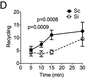
Sc: Rabenosyn-5 present
Si: Rabenosyn-5 not present
Using siRNA (small interfering RNA), transcription of Rabenosyn-5 can be prevented. The white pixels are TfR. "Sc" is a control for the siRNA function (scrambled siRNA).
Considering the TIRF images (where Sc means that Rabenosyn-5 is active because the surpressing siRNA is scrambled), it is seen that the cell has a higher TfR surface concentration compared to the case where the siRNA is active (right TIRF image). The difference is reported to be a decrease of 75% in the TIRF image. The decrease measured by EPI is less pronounced. Put differently, when Rabenosyn-5 is not produced, the TfR surface amount is reduced which also means that Tf uptake is reduced in TfR depleted cells.

This observation leads to the question, how Rabenosyn-5 controls the cell surface TfR level. Does Rabenosyn-5 regulate TfR gene transcription, TfR gene translation or some other kind of post-translational mechanism? This question is answered by panel A of Fig. 6A in the article.
Fig. 6A: http://www.pnas.org/content/109/8/E471/F6.large.jpg


GADPH is used to provide a scale for the measurement.


Possibility of translational regulation. It is known that translation of TfR can be regulated by mRNA parts before and behind the sequence coding for the protein (so called untranslated regions, UTRs).
To test for translational effects of Rabenosyn-5, the host was transfected by TfR-GFP (green fluorescent protein) lacking these UTRs (that means translation of this TfR-GFP can not be regulated). As can be seen, when Rabenosyn-5 is active (Rbsn Sc column), both TfR and TfR-GFP are produced (right most panel, Sc column). However, when Rabenosyn-5 is surpressed (right most panel, Si column) both TfR-GFP (lacking the regulatory sequences) as well as native TfR are present at lower levels.
This means Rabenosyn-5 can not be having an effect on the translation of TfR, because then TfR-GFP levels would not have been reduced (since its translation can not have been regulated)- but the TfR-GFP levels are reduced. Put differently, regulation of TfR by Rabenosyn-5 must be post-translational. So how come the TfR-GFP levels be reduced when this can not be caused by translational regulation?
Possibility of transcriptional regulation. Although there is no experiement discussing this specifically, the question, if TfR levels are regulated at the transcriptional level, is answered by considering that the gene for TfR-GFP does not contain promoter sequences. Therefore it is not possible that Rabenosyn-5 has a transcriptional effect.

Now, if not at the transcriptional nor translational level, how else can Rabenosyn-5 control TfR levels?
The hypothesis is that Rabenosyn-5 acts as a sort of label for how the cell should handle internalized TfR. Once TfR is internalized, it can be directed to the lyosome, i.e. degraded or it can be recycled, that means the TfR is returned to the cell surface and reused. The explanation for the lower levels of TfR in the absence of Rabenosyn-5 is that when Rabenosyn-5 is not present, a larger proportion of TfR gets directed towards the lysosome and subsequently degraded. Evidence for this mechanism is found in that recycling rates are significantly lower in Rabenosyn-5 deactivated cells (Fig. 5D in article).

Release rates (arbitrary units) of previously internalized Tf depending on time.
http://www.pnas.org/content/109/8/E471/F5.expansion.html
Put differently, a lower proportion gets recycled to the cell surface resulting in apparent lower TfR cell surface amount. These mechanistic alternatives are illustrated by the red arrows in the figure below (Fig. 6C in article):

Fig. 6C: Alternative mechanisms of TfR sorting in presence and absence of Rabenosyn-5.
Top panel: Rabenosyn-5 labels clathrin coated TfR vesicles for recycling (and reuse of TfR) to cell surface.
Lower panel: Absence of Rabenosyn-5 results in TfR vesicles being directed to lysosome for degrading.
http://www.pnas.org/content/109/8/E471/F6.large.jpg


This is verified by comparing TfR levels between cells with activated and deactivated lysosomes (Fig. 6B in article).
Fig. 6B: Baf: Bafilomycin A1.
Sc/Si refer to scrambled and siRNA of Rabenosyn-5.
"+": Baf present, "-": Baf absent
http://www.pnas.org/content/109/8/E471/F6.large.jpg

Under the influence of Bafilomycin A1 ("Baf") an inhibitor of lysosome operation, the TfR level is higher than when the lysosome is operational: the TfR level in the column Baf+/Sc is most intensive because it reports the TfR levels on the cell surface as well as those in the disfunctional lysosomes.

An additional finding is that the absence of Rabenosyn-5 has an effect on clathrin dynamics. In the absence of Rabenosyn-5, the number of clathrin regions and the size of the clathrin regions are increased. In the absence of Rabenosyn-5, increased clathrin signals are reported in the region of the cell nucleus (Fig. 7C in article).
Fig. 7C: left panels: Rabenosyn-5 present
right panels: Rabenosyn-5 deactivated
http://www.pnas.org/content/109/8/E471/F7.expansion.html
However, as shown in Fig. 6C, the total cellular clathrin amount is not affected by the deactivation of Rabenosyn-5. It appears therefore as if the depletion of Rabenosyn-5 results in a redistribution of clathrin, which normally is also present as unassembled clathrin in the cytoplasma, to the cell surface and to the nuclear region. It is therefore reasonable to expect that such a redistribution of clathrin at the nuclear region is only observed because a specific, directing, not yet completely characterized interaction between Rabenosyn-5 and clathrin is missing in the Rabenosyn-5 deactivated cells. The authors contemplate that when Rabenosyn-5 is missing, this results in delayed movement of cathrin coated vesicles away from the plasma membrane or a delay in their uncoating and fusion with endosomes.
Summary. The paper presents evidence for the hypothesis that Rabenosyn-5 prevents TfR from getting directed to the lysosome for degradation. The mechanism of this labeling is however yet to be characterized in detail.

Editorial. I have contacted the senior author of the paper (Prof. Corvera) to ask if she agrees to calling Rabenosyn-5 a labeling agent as stated above. Prof. Corvera added that in Rabenosyn-5 deficient mice severe perinatal phenotypes are observed. Furthermore, she added that based on this work she was approached by geneticists who have found Rabensyn-5 mutations in humans with severe neurological and developmental delays.